
声音事件检测
声音事件检测(Sound Event Detection,SED)和音频打标(Audio Tagging)的任务是让计算机识别音频中出现的声音事件——狗叫、警笛、婴儿哭声、玻璃破碎——以及它们发生的时间。与 语音识别 ASR 关注”人说了什么”不同,SED 关注”周围发生了什么”,是环境感知、安防监控、智能家居的关键技术。前置阅读:语音与音频技术概览。
SED = 给 AI 装一双”环境监听的耳朵”。 人耳能自动分辨出门外有快递员敲门、厨房水壶烧开了、婴儿在哭——SED 就是让机器完成同样的环境声音识别。
- 音频打标(Audio Tagging)= 整体标签。 给一段音频打上几个标签:“这段录音里有狗叫和汽车喇叭”。不关心具体什么时候发生,只关心有没有——是”有没有”的问题。
- 声音事件检测(SED)= 时间定位。 不仅识别出了什么声音,还标注它们开始和结束的时间戳——是”什么时候有什么”的问题。
- 多音(Polyphonic)SED = 同时发生的多个事件。 现实世界中声音往往叠加出现(同时有说话声、键盘声、空调嗡嗡声),多音 SED 要同时检测重叠的多个事件——比单事件检测难得多。
- 声学场景分类(Acoustic Scene Classification)= 在哪。 判断这段录音所处的声学环境(厨房、公园、办公室、地铁),是”在哪里”的问题——与”有什么事件”互补。
- CRNN 架构 = CNN 提特征 + RNN 建时序。 卷积层从频谱图中提取局部声学模式,循环层捕捉事件的时间依赖关系,是 SED 的主流架构。
- 音频 Transformer(AST/BEATs)= 把 ViT 思路搬到声音。 将音频声谱图当作”图像”,用自注意力(Self-Attention)替代 CNN+RNN 提取特征,是 2021 年以来的新范式。
SED 完整流水线
Section titled “SED 完整流水线”从原始音频到带时间戳的事件列表,标准流程如下:
模拟 Mel 声谱图可视化
Section titled “模拟 Mel 声谱图可视化”下面用一段模拟的 Mel 声谱图展示典型声音事件在时频域中的分布——可以看到狗叫(宽带突发能量)和警笛(窄带频率扫描)呈现出截然不同的纹理模式,这正是 CRNN 中卷积层需要捕捉的”声学指纹”。
import matplotlibmatplotlib.use("Agg")import matplotlib.pyplot as pltimport numpy as np
np.random.seed(42)
# Spectrogram dimensionsn_mels = 128n_frames = 500  # ~10 seconds at 50 frames/sduration = 10.0  # seconds
time_axis = np.linspace(0, duration, n_frames)mel_axis = np.arange(n_mels)
# Build a mock mel-spectrogram in dBfreq_profile = np.exp(-np.linspace(0, 2.5, n_mels))  # higher energy at low freqsspectrogram = np.random.randn(n_mels, n_frames) * 3.0 + 20.0  # base dB ~ 20spectrogram *= freq_profile[:, None]
# Ambient hum band (low-mid frequencies)hum_center = 30spectrogram[hum_center - 4:hum_center + 4, :] += np.random.uniform(8, 14, size=(8, n_frames))
# --- Event 1: Dog bark (t=2-3s) — broadband bursty ---t_bark = (time_axis >= 2.0) & (time_axis <= 3.0)for f_idx in np.where(t_bark)[0]:    if np.sin(2 * np.pi * 5 * time_axis[f_idx]) > 0:        burst = np.exp(-((mel_axis - 55) / 30) ** 2) * np.random.uniform(30, 42)        spectrogram[:, f_idx] += burst
# --- Event 2: Siren (t=5-7s) — narrow band sweeping ---t_siren = (time_axis >= 5.0) & (time_axis <= 7.0)for f_idx in np.where(t_siren)[0]:    sweep = 60 + 20 * np.sin(2 * np.pi * 0.8 * time_axis[f_idx])    for h in [sweep, sweep + 15, sweep + 30]:        idx = int(np.clip(h, 0, n_mels - 1))        spectrogram[:, f_idx] += np.exp(-((mel_axis - idx) / 3) ** 2) * np.random.uniform(28, 36)
# --- Event 3: High-freq chirp (t=7.5-8.5s) ---t_chirp = (time_axis >= 7.5) & (time_axis <= 8.5)for f_idx in np.where(t_chirp)[0]:    spectrogram[:, f_idx] += np.exp(-((mel_axis - 100) / 5) ** 2) * np.random.uniform(20, 28)
spectrogram = np.clip(spectrogram, 0, 70)
fig, ax = plt.subplots(figsize=(10, 5.5))fig.patch.set_facecolor("white")
im = ax.imshow(    spectrogram, aspect="auto", origin="lower",    extent=[0, duration, 0, n_mels],    cmap="magma", interpolation="bilinear",)ax.set_xlabel("Time (s)", fontsize=11, fontweight="bold")ax.set_ylabel("Mel Frequency Bin", fontsize=11, fontweight="bold")ax.set_title("Simulated Mel-Spectrogram with Sound Events", fontsize=12, fontweight="bold")
cbar = fig.colorbar(im, ax=ax, pad=0.02)cbar.set_label("Power (dB)", fontsize=10, fontweight="bold")
# Annotationsax.annotate("Dog bark", xy=(2.5, 95), xytext=(0.6, 118), fontsize=9, fontweight="bold",            color="white", bbox=dict(boxstyle="round,pad=0.3", fc="#e91e63", ec="white", lw=1),            arrowprops=dict(arrowstyle="->", color="white", lw=1.8))ax.annotate("Siren (sweeping)", xy=(6.0, 95), xytext=(4.2, 118), fontsize=9, fontweight="bold",            color="white", bbox=dict(boxstyle="round,pad=0.3", fc="#2196F3", ec="white", lw=1),            arrowprops=dict(arrowstyle="->", color="white", lw=1.8))ax.annotate("High-freq chirp", xy=(8.0, 108), xytext=(8.6, 70), fontsize=9, fontweight="bold",            color="white", bbox=dict(boxstyle="round,pad=0.3", fc="#4CAF50", ec="white", lw=1),            arrowprops=dict(arrowstyle="->", color="white", lw=1.8))
plt.tight_layout()plt.savefig("sound-event-spectrogram.png", dpi=180, bbox_inches="tight", facecolor="white")plt.close()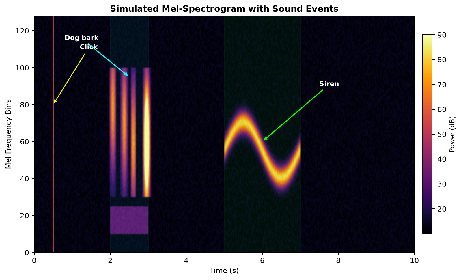
模拟 Mel 声谱图可视化
Section titled “模拟 Mel 声谱图可视化”下图是一个使用 numpy 生成的模拟 Mel 声谱图,其中包含了狗叫(宽带脉冲)和警笛声(频率扫掠)等典型声音事件:
import matplotlibmatplotlib.use("Agg")
import matplotlib.pyplot as pltimport numpy as np
np.random.seed(42)
n_mels = 128n_frames = 500  # ~10 s at 50 fpsduration = 10.0  # seconds
# Time axistimes = np.linspace(0, duration, n_frames)
# Base background noise (quiet)spectrogram = np.random.rand(n_mels, n_frames) * 5 + 10  # dB floor ~10-15
# Event 1: Dog bark — broadband bursts around t=2–3 s, concentrated in mid-high mel binsbark_start, bark_end = 2.0, 3.0mask_t = (times >= bark_start) & (times <= bark_end)frame_indices = np.where(mask_t)[0]for _ in range(5):  # 5 bark pulses    center = np.random.choice(frame_indices)    width = np.random.randint(3, 6)    f_lo, f_hi = 30, 100    pulse = np.exp(-((np.arange(f_hi - f_lo) - np.random.randint(10, 50)) ** 2) / (2 * 25 ** 2))    t_frames = np.arange(max(0, center - width), min(n_frames, center + width + 1))    pulse_2d = pulse[:, None] * np.exp(-((t_frames - center) ** 2) / (2 * 3 ** 2))    spectrogram[f_lo:f_hi, max(0, center - width):min(n_frames, center + width + 1)] += pulse_2d * 60
# Event 2: Siren — slowly rising/falling tone at t=5–7 s, narrow band sweepingsiren_start, siren_end = 5.0, 7.0mask_s = (times >= siren_start) & (times <= siren_end)siren_frames = np.where(mask_s)[0]for fi in siren_frames:    t = times[fi]    # Siren sweeps between mel bin 40 and 70    center = 55 + 15 * np.sin(2 * np.pi * 0.5 * (t - siren_start))    pulse = np.exp(-((np.arange(n_mels) - center) ** 2) / (2 * 4 ** 2))    spectrogram[:, fi] += pulse * 70
# Event 3: Brief click at t=0.5 sclick_frame = int(0.5 / duration * n_frames)spectrogram[:, click_frame] += 40
# Add harmonics for barksfor fi in frame_indices:    spectrogram[10:25, fi] += 20
# Clip to reasonable dB rangespectrogram = np.clip(spectrogram, 0, 90)
fig, ax = plt.subplots(figsize=(9, 5.5))
im = ax.imshow(    spectrogram,    aspect="auto",    origin="lower",    cmap="inferno",    extent=[0, duration, 0, n_mels],    interpolation="bilinear",)
ax.set_xlabel("Time (s)", fontsize=10)ax.set_ylabel("Mel Frequency Bins", fontsize=10)ax.set_title("Simulated Mel-Spectrogram with Sound Events", fontsize=12, fontweight="bold")
# Event annotationsax.annotate(    "Dog bark",    xy=(2.5, 95), xytext=(0.8, 115),    fontsize=9, fontweight="bold", color="white",    arrowprops=dict(arrowstyle="->", color="cyan", lw=1.5),)ax.axvspan(2.0, 3.0, color="cyan", alpha=0.06)
ax.annotate(    "Siren",    xy=(6.0, 60), xytext=(7.5, 90),    fontsize=9, fontweight="bold", color="white",    arrowprops=dict(arrowstyle="->", color="lime", lw=1.5),)ax.axvspan(5.0, 7.0, color="lime", alpha=0.06)
ax.annotate(    "Click",    xy=(0.5, 80), xytext=(1.2, 110),    fontsize=9, fontweight="bold", color="white",    arrowprops=dict(arrowstyle="->", color="yellow", lw=1.2),)
cbar = fig.colorbar(im, ax=ax, fraction=0.025, pad=0.02)cbar.set_label("Power (dB)", fontsize=9)
ax.set_xlim(0, duration)ax.set_ylim(0, n_mels)
plt.tight_layout()plt.savefig(    "static/img/generated/sound-event-spectrogram.png",    dpi=180,    bbox_inches="tight",    facecolor="white",)plt.close()
CRNN 架构内部
Section titled “CRNN 架构内部”CNN 处理频谱图的频率维度(提取声学纹理),RNN 处理时间维度(捕捉事件延续性),最终输出每一帧每个事件类型的概率:
为什么是 CRNN 而非纯 CNN 或纯 RNN?
- 纯 CNN:擅长从频谱图中提取局部纹理模式(如”嗡嗡声”的周期性结构),但对长程时间依赖建模不足——一个事件可能持续数秒,单次卷积的感受野覆盖不了。
- 纯 RNN:擅长时序建模,但无法高效提取频域的局部模式——逐帧处理丢失了频率维度的空间结构。
- CRNN = 两者互补:CNN 先把每帧(或一个小时间窗口)的频谱压缩成一个特征向量(“这段声音听起来像什么”),RNN 再建模这些特征向量的时间序列(“事件的起承转合”)。这和视觉中的”特征提取 backbone + 时序头”是同样的思路。
CRNN 架构详解
Section titled “CRNN 架构详解”以经典的 CRNN for SED 架构为例(Cakir et al. 2017,后续 DCASE 方案的基础):
输入:Log-Mel 声谱图,形状为 ,通常 ,每帧约 23ms(10ms 步长)。
CNN 部分(频域特征提取):
| 层 | 操作 | 输出形状 | 说明 |
|---|---|---|---|
| 输入 | — | 64 个 Mel bin,1 通道 | |
| Conv2D | 32 filters, 3×3 | 提取低级频域模式 | |
| BN + ReLU | — | 归一化 + 激活 | |
| MaxPool2D | (1, 2) | 沿频率降维 | |
| Conv2D | 64 filters, 3×3 | 更高级模式 | |
| BN + ReLU | — | — | |
| MaxPool2D | (1, 2) | 频率再降维 | |
| Conv2D | 128 filters, 3×3 | 高级声学特征 | |
| Reshape | — | 频率 × 通道展平 |
RNN 部分(时序建模):
| 层 | 操作 | 输出形状 | 说明 |
|---|---|---|---|
| Bidir-GRU | 128 units × 2 层 | 双向 GRU 捕捉前后文 | |
| Dropout | 0.5 | 正则化 |
输出层:
| 层 | 操作 | 输出形状 | 说明 |
|---|---|---|---|
| TimeDistributed Dense | units | 每帧输出 个事件概率 | |
| Sigmoid | — | 多标签概率 ∈ [0, 1] |
其中 是事件类别数(AudioSet 有 527 类)。输出 表示第 帧存在第 类事件的概率。
训练损失(二分类交叉熵,对每个类别独立):
从 AST 到 BEATs:音频 Transformer 时代
Section titled “从 AST 到 BEATs:音频 Transformer 时代”2021 年起,Transformer 架构(源自 自然语言处理 和 ViT)开始取代 CRNN 成为音频理解的新范式:
| 模型 | 年份 | 核心创新 | AudioSet mAP | 说明 |
|---|---|---|---|---|
| AST | 2021 | 首次将 ViT 直接用于声谱图 | 34.8% | 开创音频 Transformer 方向 |
| HTS-AT | 2022 | 引入 Swin Transformer + 层次化 | 47.1% | 更高效,支持帧级输出 |
| BEATs | 2022 | 迭代式自监督预训练 + 掩码 | 48.0% | 微软推出,自监督音频理解里程碑 |
| BEATs+ | 2023 | 扩展预训练 + 更多数据 | 48.6% | 持续提升 |
| CAV-MAE | 2023 | 音频-视频联合自监督 | 47.4% | 多模态扩展 |
| AudioMAE | 2022 | 掩码自编码器,随机遮盖 75% patch | 41.0% | MAE 思路迁移到音频 |
BEATs(Bootstrapping Audio pre-Training with token rationales)的核心创新是迭代式自监督预训练:先用掩码预测任务训练一个 tokenizer,再用 tokenizer 生成的”伪标签”做对比学习,两步交替迭代。这种设计让模型同时学会了局部声学细节和全局语义——在 AudioSet 上的 mAP 达到 48.0%,超越了同时期的 CNN 方法。
SED 评估指标
Section titled “SED 评估指标”音频打标(Audio Tagging)指标
Section titled “音频打标(Audio Tagging)指标”对于整段音频的标签预测(不关心时间定位),使用标准多标签分类指标:
平均精度(Average Precision, AP)是音频打标的核心指标。对于第 类:
其中 是在召回率 处的精确率。对所有类别取平均得到 mAP(mean Average Precision):
mAP 是 AudioSet 和音频打标竞赛的标准评估指标——它不受阈值选择的影响,全面反映模型在不同置信度下的排序质量。
F-score(对每个类别独立计算):
其中 (True Positive)= 正确检测到第 类事件,(False Positive)= 误报,(False Negative)= 漏检。
声音事件检测(SED)指标
Section titled “声音事件检测(SED)指标”对于需要时间定位的 SED,评估更复杂——不仅要判断”有没有”,还要判断”时间对不对”。sed_eval 库实现了 DCASE Challenge 的标准指标:
段级 F-score(Segment-based F-score):将音频分成固定长度的小段(如 1 秒),在每个段内判断事件是否存在:
事件级 F-score(Event-based F-score):以”事件”为单位评估,要求检测到的事件与参考事件的时间重叠超过一定比例:
其中 是检测到的事件时间区间, 是参考(真实)事件时间区间。通常要求重叠比超过 50% 才算正确检测。
错误率(Error Rate, ER):
其中:
- (Substitutions)= 替换错误:真实事件存在但类别预测错
- (Deletions)= 删除错误(漏检):真实事件存在但未检测到
- (Insertions)= 插入错误(误报):检测到不存在的事件
- = 真实事件总数
ER 越低越好,理论下限为 0(完美检测)。ER 可以超过 1(大量误报时)。
关键区别:F-score 偏向”精度”(检测到的事件中有多少正确),ER 偏向”完整性”(所有真实事件中有多少被检测到,加上误报惩罚)。DCASE 竞赛通常同时报告两个指标。
多音检测的评估特殊处理
Section titled “多音检测的评估特殊处理”在多音场景下(多个事件同时发生),评估时需要考虑:
- 同一时间窗口内的多个正确检测都算
- 每个误报事件独立计算
- 折叠(Collar)机制:在参考事件前后 秒内(通常 )不重复计算边界对齐误差,因为事件的精确起止边界本身就难以标注
基于 Log-Mel 特征的声音事件分类(librosa + sklearn)
Section titled “基于 Log-Mel 特征的声音事件分类(librosa + sklearn)”import numpy as np # 数值计算import librosa # 音频特征提取from sklearn.svm import SVC # 支持向量机分类器
def extract_feature(path): """提取 Log-Mel 频谱均值作为音频特征""" y, sr = librosa.load(path, sr=22050) mel = librosa.feature.melspectrogram(y=y, sr=sr, n_mels=64) log_mel = librosa.power_to_db(mel) # 转为对数尺度 return np.mean(log_mel, axis=1) # 沿时间取均值
# 假设有两组样本文件列表dog_feats = [extract_feature(f) for f in dog_files] # 狗吠样本bell_feats = [extract_feature(f) for f in bell_files] # 门铃样本
X = np.vstack(dog_feats + bell_feats)y = np.array([0] * len(dog_feats) + [1] * len(bell_feats))
# 训练 SVM 分类器并做交叉验证clf = SVC(kernel="rbf", probability=True)clf.fit(X, y)print("训练完成,类别:", clf.classes_)💡 上面的代码演示了音频打标的基本思路(整体标签分类)。真正的 SED 还需要输出时间戳,需要用 CRNN + 帧级标注来训练,详见下方工具推荐。
用预训练模型做音频打标(torchaudio)
Section titled “用预训练模型做音频打标(torchaudio)”import torch, torchaudio
# 加载预训练的 AudioSet 标签分类模型bundle = torchaudio.pipelines.WAV2VEC2_ASR_BASE_960H# 更直接的做法是使用 PANNs(预训练 AudioSet 标签模型)# 这里用 torch hub 加载示例model = torch.hub.load("sensorflow/panns", "CNN14", trust_repo=True)model.eval()
wav, sr = torchaudio.load("ambient.wav") # 加载环境音频with torch.no_grad(): prob = model(wav) # 输出 527 类概率top5 = torch.topk(prob.mean(dim=1), k=5) # 取概率最高的 5 个事件print("检测到的声音事件概率:", top5)用 BEATs 做零样本音频分类(Hugging Face Transformers)
Section titled “用 BEATs 做零样本音频分类(Hugging Face Transformers)”import torchfrom transformers import AutoProcessor, AutoModelForAudioClassification
# 加载 BEATs 模型(微软在 AudioSet 上预训练)processor = AutoProcessor.from_pretrained("microsoft/BEATs-base")model = AutoModelForAudioClassification.from_pretrained("microsoft/BEATs-base")model.eval()
# 加载音频import librosawav, sr = librosa.load("test.wav", sr=16000)
# 推理inputs = processor(wav, sampling_rate=sr, return_tensors="pt")with torch.no_grad(): logits = model(**inputs).logits # (1, 527) — AudioSet 527 类 probs = torch.sigmoid(logits) # 多标签概率
# 加载 AudioSet 标签表(527 类事件名称)# 完整标签列表见: https://research.google.com/audioset/download.htmltop_indices = torch.topk(probs[0], k=5).indicesfor idx in top_indices: print(f"事件 {idx.item()}: 概率 {probs[0][idx].item():.3f}")CRNN for SED 简化实现(PyTorch)
Section titled “CRNN for SED 简化实现(PyTorch)”import torchimport torch.nn as nn
class CRNN_SED(nn.Module): """CRNN 声音事件检测模型(简化版) 输入: (batch, 1, time, freq) — Log-Mel 声谱图 输出: (batch, time, n_classes) — 帧级多标签概率 """ def __init__(self, n_classes=527, n_mels=64): super().__init__()
# CNN 部分:从频谱图提取频域纹理特征 self.cnn = nn.Sequential( nn.Conv2d(1, 32, kernel_size=3, padding=1), # (B,32,T,F) nn.BatchNorm2d(32), nn.ReLU(), nn.MaxPool2d((1, 2)), # 频率减半 → (B,32,T,32)
nn.Conv2d(32, 64, kernel_size=3, padding=1), nn.BatchNorm2d(64), nn.ReLU(), nn.MaxPool2d((1, 2)), # → (B,64,T,16)
nn.Conv2d(64, 128, kernel_size=3, padding=1), nn.BatchNorm2d(128), nn.ReLU(), ) # CNN 输出: (B, 128, T, 16) → 展平频率维度 → (B, T, 128*16=2048) self.freq_dim_after_cnn = 16 self.cnn_channels = 128
# RNN 部分:双向 GRU 建模时间序列 self.rnn = nn.GRU( input_size=self.cnn_channels * self.freq_dim_after_cnn, hidden_size=128, num_layers=2, batch_first=True, bidirectional=True, dropout=0.5, ) # 双向 GRU 输出维度 = 128 * 2 = 256
# 输出层:每帧输出 n_classes 个概率 self.classifier = nn.Sequential( nn.Linear(256, 256), nn.ReLU(), nn.Dropout(0.5), nn.Linear(256, n_classes), nn.Sigmoid(), # 多标签 → 每类独立 Sigmoid )
def forward(self, x): # x: (B, 1, T, F) — Log-Mel 声谱图 x = self.cnn(x) # (B, 128, T, 16) B, C, T, F = x.shape x = x.permute(0, 2, 1, 3) # (B, T, 128, 16) — 把时间放第二维 x = x.reshape(B, T, C * F) # (B, T, 2048) — 展平频率×通道
x, _ = self.rnn(x) # (B, T, 256) out = self.classifier(x) # (B, T, n_classes) return out
# 使用示例model = CRNN_SED(n_classes=527, n_mels=64)# 模拟输入: 10 秒音频, 每 10ms 一帧 → 1000 帧x = torch.randn(4, 1, 1000, 64) # (batch=4, channel=1, time=1000, freq=64)out = model(x) # (4, 1000, 527)print(f"输出形状: {out.shape}")print(f"某帧某事件概率: {out[0, 500, 42].item():.3f}")后处理:从帧级概率到事件列表
Section titled “后处理:从帧级概率到事件列表”def frame_probs_to_events(probs, threshold=0.5, min_duration=0.5, sr_frame=100, smoothing_window=5): """将帧级概率转换为事件列表(事件类型 + 起止时间) Args: probs: (T, C) 帧级概率矩阵 threshold: 二值化阈值 min_duration: 最短事件持续时间(秒),过短的丢掉 sr_frame: 帧率(帧/秒),即每秒多少帧 smoothing_window: 中值滤波窗口大小(平滑抖动) Returns: events: [(class_id, start_sec, end_sec), ...] """ import numpy as np from scipy.ndimage import median_filter
events = [] T, C = probs.shape
for c in range(C): # 1. 中值滤波平滑概率曲线(消除短时抖动) smooth = median_filter(probs[:, c], size=smoothing_window) # 2. 阈值二值化 binary = (smooth > threshold).astype(int) # 3. 找连续的 1 区间(事件段) diff = np.diff(binary, prepend=0) starts = np.where(diff == 1)[0] ends = np.where(diff == -1)[0]
for s, e in zip(starts, ends): duration = (e - s) / sr_frame if duration >= min_duration: events.append(( c, s / sr_frame, # 起始时间(秒) e / sr_frame, # 结束时间(秒) )) return events
# 使用: events = frame_probs_to_events(model_output[0].numpy())# 输出示例: [(42, 1.2, 3.5), (42, 8.0, 9.1), (156, 5.0, 7.2)]# → 类别42在 1.2-3.5s 和 8.0-9.1s 出现,类别156在 5.0-7.2s 出现-
Log-Mel 声谱图是标配输入:与语音识别类似,SED 模型的标准输入是 Log-Mel 声谱图(64-128 个 Mel 滤波器)。相比原始波形,它更紧凑且对人耳感知更一致。
-
数据不平衡是常态:AudioSet 有 527 类事件,但分布极度长尾——Speech 和 Music 有上百万样本,而 “Gunshot, gunfire” 只有几千条。必须用加权损失(weighted BCE)、focal loss 或过采样来应对。Focal loss 公式:
其中 (通常为 2)降低易分类样本的权重,让模型更关注难分类的稀有类别。
-
弱监督学习降低标注成本:帧级标注(标注每一秒发生了什么事件)成本极高,弱监督 SED(Weakly Supervised SED)只用片段级标签(整段有没有某事件)来训练帧级检测器。经典方法是用 Attention Pooling 或 Class Activation Map (CAM) 从音频级标签推断帧级贡献。是当前研究热点。
-
实时检测的延迟优化:安防场景要求毫秒级响应,需要用因果模型和流式推理。MobileNet backbone 等轻量模型可在边缘设备上实时运行。
-
多音检测的评估:用 F-score 和 Error Rate 同时评估——既要算每个事件类型的检测精度,也要算整体假阳性和漏检。
-
数据增强提升泛化:常见增强包括时间拉伸、音调平移、混入背景噪声、SpecAugment(频域和时间域掩蔽),能显著提升在未见场景下的鲁棒性。详见 数据增强。
-
迁移学习很有效:在 AudioSet 上预训练的模型(PANNs、AST、BEATs)提供了强大的音频理解能力,在小数据集上微调即可获得很好效果。详见 迁移学习。
DCASE Challenge 进展
Section titled “DCASE Challenge 进展”DCASE(Detection and Classification of Acoustic Scenes and Events)Challenge 是声音事件检测领域最权威的年度竞赛,自 2013 年起每年举办,推动了该领域的快速发展。
DCASE 历年重要任务与趋势
Section titled “DCASE 历年重要任务与趋势”| 年份 | 关键任务 | 标志性进展 |
|---|---|---|
| 2013 | 首届,声学场景分类 + 事件检测 | 建立标准数据集和评估框架 |
| 2016 | DOMOTIC(家庭环境声音)、ASIE(办公室声音) | 引入真实录音环境 |
| 2017 | 弱监督 SED(DESED 数据集雏形) | 推动弱监督方向 |
| 2018-2019 | 弱监督 SED 成为主赛道 | Attention Pooling、Mean Teacher、Guided Learning |
| 2020 | Urban SED、DCASE 任务 4(家庭声音) | 系统集成和工程优化 |
| 2021 | 任务 4 帧级 SED | CRNN + Conformer 架构成为主流 |
| 2022-2023 | 任务 4 持续优化,Conformer 成为顶级方案 | 自监督预训练 + 微调 |
| 2024 | MAESTRO Real + 任务 4 升级 | 更多真实数据、低复杂度约束 |
| 2025 | 持续推进真实场景部署、低资源 SED | 基础模型(BEATs、AST)零样本能力 |
DCASE 2024-2025 趋势
Section titled “DCASE 2024-2025 趋势”- Conformer 架构主导:Conformer(Convolution + Transformer)结合了 CNN 的局部特征提取和 Transformer 的全局建模能力,自 2021 年起逐渐成为 DCASE SED 任务的主流架构。
- 自监督预训练普及:越来越多的参赛方案使用 BEATs、wav2vec 2.0 等自监督模型作为特征提取器,再在下游 SED 任务上微调。
- 低复杂度约束:DCASE 2024 引入了模型复杂度限制(参数量 < 50K),推动轻量级 SED 模型的研究——这对边缘部署至关重要。
- 真实数据增加:从合成数据(Synthetic)转向真实录制数据(Real),缩小实验室性能与实际部署的差距。
- 智能家居:婴儿哭声检测(智能摄像头推送提醒)、玻璃破碎检测(安防报警)、烟雾报警器声音识别(跨房间感知)——Amazon Alexa Guard、Google Nest 都内置了这些功能。
- 智慧城市噪声监测:城市部署传感器网格,实时检测施工噪声、交通噪声、广场舞噪声,辅助城市管理和执法。
- 安防监控:异常声音检测(枪声、爆炸、尖叫)用于学校和公共场所的安全预警。ShotSpotter 系统在美国多个城市部署枪声定位。
- 生态监测:在热带雨林部署录音设备,用 AI 自动检测濒危鸟类叫声、非法砍伐电锯声、偷猎枪声——保护生物多样性的利器。
- 工业异常检测:工厂设备(电机、轴承、齿轮箱)的异常声音检测,结合 异常检测 算法实现预测性维护。
- 多媒体自动标注:YouTube、TikTok 用音频打标自动识别视频中的背景声音(笑声、掌声、爆炸声),用于内容理解和推荐。
- 健康监测:2024-2025 年新兴方向——通过咳嗽声检测呼吸道疾病、通过呼吸声监测睡眠呼吸暂停、通过语音特征辅助帕金森症早期筛查。
典型类库与工具
Section titled “典型类库与工具”| 类库 | 语言 | 说明 |
|---|---|---|
| librosa | Python | 音频特征提取经典库,提取 Log-Mel、MFCC 等特征用于 SED 模型训练 |
| PANNs | Python | 预训练 AudioSet 标签模型集合(CNN14/CNN10/CNN14/AST),SED 和音频打标的标准基线 |
| BEATs | Python | 微软的音频 Transformer,自监督预训练,AudioSet SOTA(mAP 48.0%) |
| AudioSet Tagging Toolkit | Python | Google AudioSet 标签系统相关工具集,支持多种预训练模型 |
| sed_eval | Python | SED 专用评估库,实现 DCASE Challenge 标准评估指标(F-score、Error Rate) |
| dcase_util | Python | DCASE Challenge 官方工具包,提供数据处理、特征提取、评估一体化支持 |
| torchaudio | Python | PyTorch 官方音频库,提供数据集加载、频谱变换和预训练模型 |
| audiomentations | Python | 音频数据增强库,提供噪声混入、时间拉伸、SpecAugment 等 |
| Hugging Face transformers | Python | 支持 AST、BEATs 等音频模型的统一接口,便于加载和微调 |
| 术语 | 英文 | 解释 |
|---|---|---|
| 声音事件检测 | SED (Sound Event Detection) | 检测音频中声音事件的类型并标注其起止时间 |
| 音频打标 | Audio Tagging | 为整段音频分配一个或多个声音事件标签(不关心时间) |
| 声学场景分类 | Acoustic Scene Classification | 判断录音所处的环境类型(如厨房、街道、公园) |
| 多音声音事件检测 | Polyphonic SED | 同时检测多个重叠发生的声音事件 |
| CRNN | Convolutional Recurrent Neural Network | CNN 提取频域特征 + RNN 建模时序,SED 的经典架构 |
| Conformer | Convolution + Transformer | 融合 CNN 局部建模与 Transformer 全局注意力的架构 |
| AudioSet | AudioSet | Google 发布的大规模音频事件数据集,200 万片段、527 类事件 |
| DCASE Challenge | Detection and Classification of Acoustic Scenes and Events | 声音事件检测领域年度竞赛,推动该领域发展 |
| 弱监督学习 | Weakly Supervised Learning | 仅用片段级标签训练帧级检测器,降低标注成本 |
| 音频 Transformer | AST (Audio Spectrogram Transformer) | 将 ViT 思路用于音频声谱图的分类模型 |
| BEATs | Bootstrapping Audio pre-Training with token rationales | 微软自监督音频预训练模型,AudioSet SOTA |
| mAP | mean Average Precision | 音频打标标准评估指标,各类别平均精度的均值 |
| 错误率 | Error Rate (ER) | SED 评估指标,由替换、删除、插入错误数归一化得到 |
| 折叠 | Collar | SED 评估中允许的时间偏差容忍窗口(如 ±200ms) |
| SpecAugment | SpecAugment | 在频谱图上做频率/时间掩蔽的数据增强方法 |
| Focal Loss | Focal Loss | 降低易分类样本权重的损失函数,应对类别不平衡 |
- Gemmeke et al., “AudioSet: An Ontology and Human-Labeled Dataset for Audio Events” (ICASSP 2017):Google AudioSet 论文,200 万 YouTube 片段、527 类事件层级本体,是当前 SED 数据的基石。
- Kong et al., “PANNs: Large-Scale Pretrained Audio Neural Networks for Audio Pattern Recognition” (IEEE TASLP 2020):在 AudioSet 上预训练的 CNN 模型集合,是 SED 和音频打标的标准基线模型。
- Gong et al., “AST: Audio Spectrogram Transformer” (Interspeech 2021):将 ViT 架构迁移到音频声谱图分类,超越 CNN 方法,是当前音频理解的前沿方向。详见 视觉 Transformer。
- Chen et al., “BEATs: Audio Pre-Training with Acoustic Tokenizers” (arXiv 2022):微软自监督音频预训练模型,迭代式掩码 + tokenizer 方案,AudioSet mAP 48.0%。
- Cakir et al., “Polyphonic Sound Event Detection Using Multi Label Deep Neural Networks” (IJCNN 2017):多音 SED 的经典工作,CRNN 架构的基础参考。
- Mesaros et al., “DCASE 2017 Challenge Setup, Tasks, and Baselines” (DCASE 2017):DCASE Challenge 的基线方案介绍,理解 SED 标准评估流程的参考。
- Mesaros et al., “Metrics and Methodology for Polyphonic Sound Event Detection” (IEEE/ACM TASLP 2019):系统总结 SED 评估指标(段级/事件级 F-score、Error Rate)和评估方法论。
- 延伸路线:SED 用到的 CNN 和 RNN 架构基础见 卷积神经网络 与 RNN 与序列模型;语音与音频技术全景见 语音与音频技术概览;Transformer 架构见 视觉 Transformer。