用代码讲解单应性矩阵的基本概念

本教程将借助一些代码演示单应性矩阵（homography）的基本概念。 关于理论的详细解释，请参阅计算机视觉课程或计算机视觉书籍，例如：

• Multiple View Geometry in Computer Vision，Richard Hartley 与 Andrew Zisserman 著，[HartleyZ00（部分样章可在此处获取，CVPR] 教程可在此处获取）
• An Invitation to 3-D Vision: From Images to Geometric Models，Yi Ma、Stefano Soatto、Jana Kosecka 与 S. Shankar Sastry 著，[Ma:2003:IVI（计算机视觉书籍讲义可在此处获取）]
• Computer Vision: Algorithms and Applications，Richard Szeliski 著，[RS10（电子版可在此处获取）]
• Deeper understanding of the homography decomposition for vision-based control，Ezio Malis、Manuel Vargas 著，[Malis2007（开放获取此处）]
• Pose Estimation for Augmented Reality: A Hands-On Survey，Eric Marchand、Hideaki Uchiyama、Fabien Spindler 著，[Marchand16（开放获取此处）]

本教程的代码可在以下地址找到：C++、 Python、 Java。 本教程使用的图像可在此处找到（left*.jpg）。

基础理论

什么是单应性矩阵？

简而言之，平面单应性矩阵描述的是两个平面之间的变换（相差一个尺度因子）：

$$s \begin{bmatrix} x^{'} \\ y^{'} \\ 1 \end{bmatrix} = \mathbf{H} \begin{bmatrix} x \\ y \\ 1 \end{bmatrix} = \begin{bmatrix} h_{11} & h_{12} & h_{13} \\ h_{21} & h_{22} & h_{23} \\ h_{31} & h_{32} & h_{33} \end{bmatrix} \begin{bmatrix} x \\ y \\ 1 \end{bmatrix}$$

单应性矩阵是一个 3x3 矩阵，但由于它是相差一个尺度估计出来的，因此只有 8 个自由度（DoF）。通常对其进行归一化（另见 \ref lecture_16 “1”）， 令 $h_{33} = 1$，或者令 $h_{11}^2 + h_{12}^2 + h_{13}^2 + h_{21}^2 + h_{22}^2 + h_{23}^2 + h_{31}^2 + h_{32}^2 + h_{33}^2 = 1$。

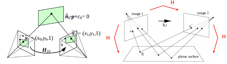
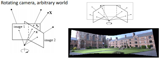
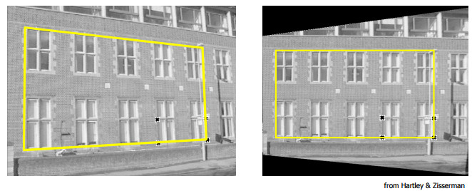
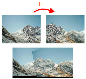
以下示例展示了不同类型的变换，但它们都描述了两个平面之间的变换关系。

• 一个平面与图像平面（图像取自 \ref projective_transformations “2”）

• 由两个相机位置观察到的同一平面（图像取自 \ref szeliski “3” 与 \ref projective_transformations “2”）

• 相机绕其投影轴旋转，等价于将这些点视为位于无穷远处的平面上（图像取自 \ref projective_transformations “2”）

单应性变换有什么用处？

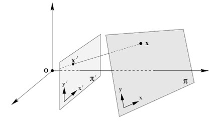
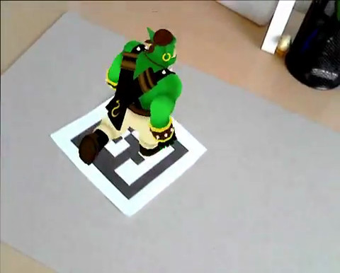
• 由共面点进行相机位姿估计，例如用于带有标记的增强现实（见前面第一个示例）

• 透视去除 / 校正（见前面第二个示例）

• 全景拼接（见前面第二个和第三个示例）

示例代码

示例 1：由共面点估计位姿

\note 请注意，由单应性矩阵估计相机位姿的代码只是一个示例；如果你想估计平面物体或任意物体的相机位姿，应当改用 cv::solvePnP。

单应性矩阵可以用例如直接线性变换（Direct Linear Transform，DLT）算法来估计（更多信息见 \ref lecture_16 “1”）。 由于物体是平面的，物体坐标系下的点与投影到图像平面（以归一化相机坐标系表示）上的点之间的变换就是一个单应性矩阵。 正是因为物体是平面的，在已知相机内参的情况下（见 \ref projective_transformations “2” 或 \ref answer_dsp “4”）， 才能从单应性矩阵中恢复出相机位姿。 这很容易用一个棋盘物体以及 findChessboardCorners() 获取图像中的角点位置来测试。

第一步是检测棋盘角点，这需要棋盘尺寸（patternSize），此处为 9x6：

已知棋盘方格的尺寸，就可以很容易地计算出物体坐标系下的物体点：

在单应性矩阵估计部分，必须去掉坐标 Z=0：

归一化相机坐标系下的图像点可由角点计算得到，方法是利用相机内参与畸变系数做逆向透视变换：

然后可以用以下方式估计单应性矩阵：

从单应性矩阵恢复位姿的一个快速解法是（见 \ref pose_ar “5”）：

$$\begin{align*} \mathbf{X} &= \left( X, Y, 0, 1 \right ) \\ \mathbf{x} &= \mathbf{P}\mathbf{X} \\ ```cpp &= \mathbf{K} \left[ \mathbf{r_1} \hspace{0.5em} \mathbf{r_2} \hspace{0.5em} \mathbf{r_3} \hspace{0.5em} \mathbf{t} \right ] ``` \begin{pmatrix} X \\ Y \\ 0 \\ 1 \end{pmatrix} \\ ```cpp &= \mathbf{K} \left[ \mathbf{r_1} \hspace{0.5em} \mathbf{r_2} \hspace{0.5em} \mathbf{t} \right ] ```   \begin{pmatrix} X \\ Y \\ 1 \end{pmatrix} \\ &= \mathbf{H} \begin{pmatrix} X \\ Y \\ 1 \end{pmatrix} \end{align*}$$ $$\begin{align*} \mathbf{H} &= \lambda \mathbf{K} \left[ \mathbf{r_1} \hspace{0.5em} \mathbf{r_2} \hspace{0.5em} \mathbf{t} \right ] \\ \mathbf{K}^{-1} \mathbf{H} &= \lambda \left[ \mathbf{r_1} \hspace{0.5em} \mathbf{r_2} \hspace{0.5em} \mathbf{t} \right ] \\ \mathbf{P} &= \mathbf{K} \left[ \mathbf{r_1} \hspace{0.5em} \mathbf{r_2} \hspace{0.5em} \left( \mathbf{r_1} \times \mathbf{r_2} \right ) \hspace{0.5em} \mathbf{t} \right ] \end{align*}$$

这是一个快速解法（另见 \ref projective_transformations “2”），因为它并不能保证得到的旋转矩阵是正交的，而且尺度只是通过将第一列归一化为 1 来粗略估计的。

要得到一个正确的旋转矩阵（具备旋转矩阵的性质），可以对旋转矩阵做极分解（polar decomposition）或正交化 （相关信息见 \ref polar_decomposition “6”、\ref polar_decomposition_svd “7”、\ref polar_decomposition_svd_2 “8” 或 \ref Kabsch_algorithm “9”）：

为了检验结果，将用估计的相机位姿把物体坐标系投影到图像上并显示出来：

示例 2：透视校正

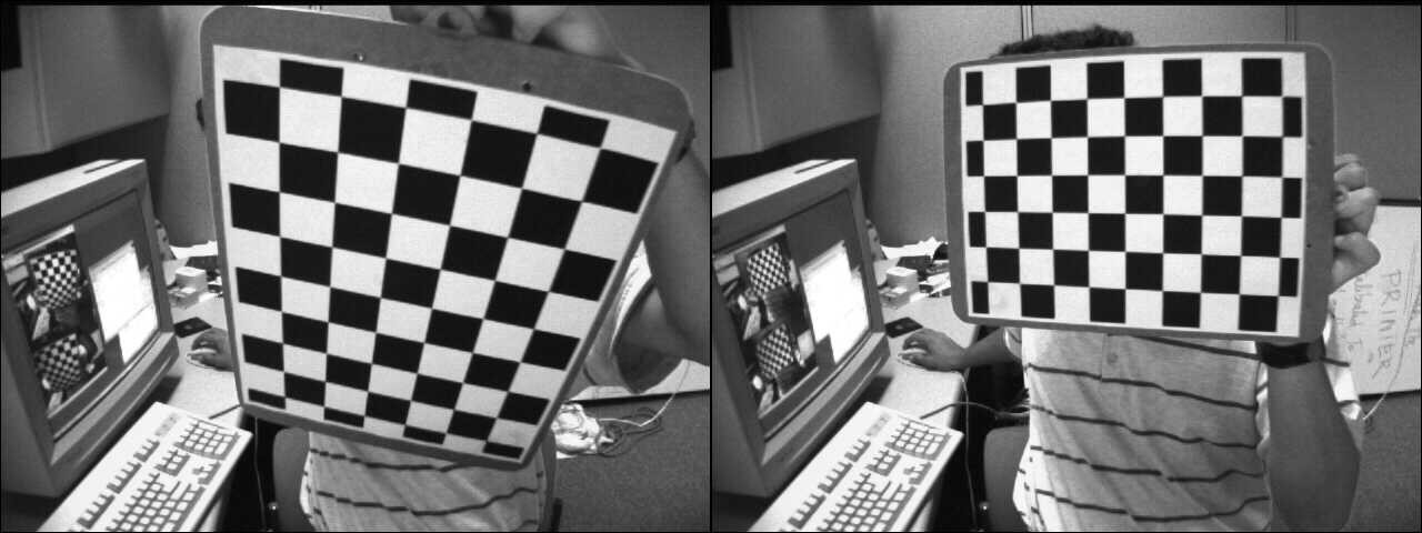
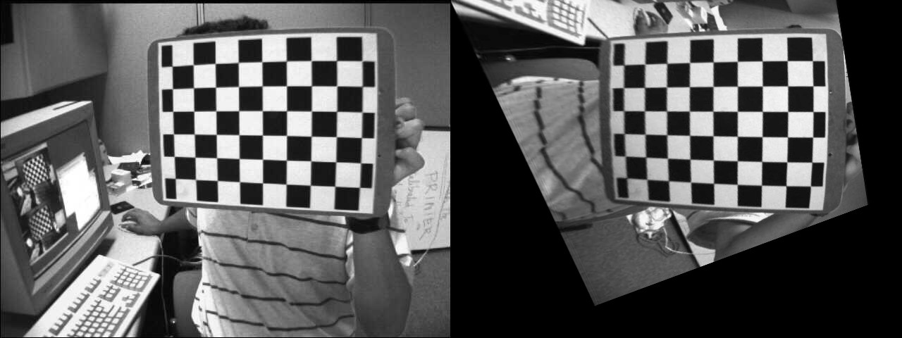
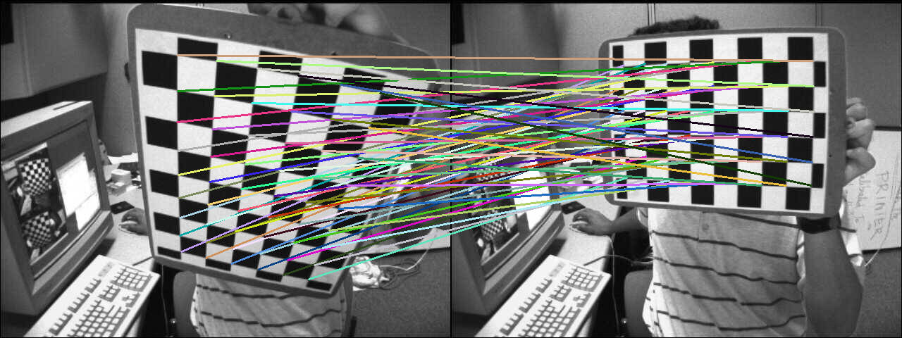
在本示例中，通过计算将源点映射到目标点的单应性矩阵，将一幅源图像变换为期望的透视视图。 下图展示了源图像（左）以及我们想要变换为期望棋盘视图的棋盘视图（右）。

第一步是在源图像和目标图像中检测棋盘角点：

单应性矩阵很容易用以下方式估计：

要将源棋盘视图变换为目标棋盘视图，我们使用 cv::warpPerspective

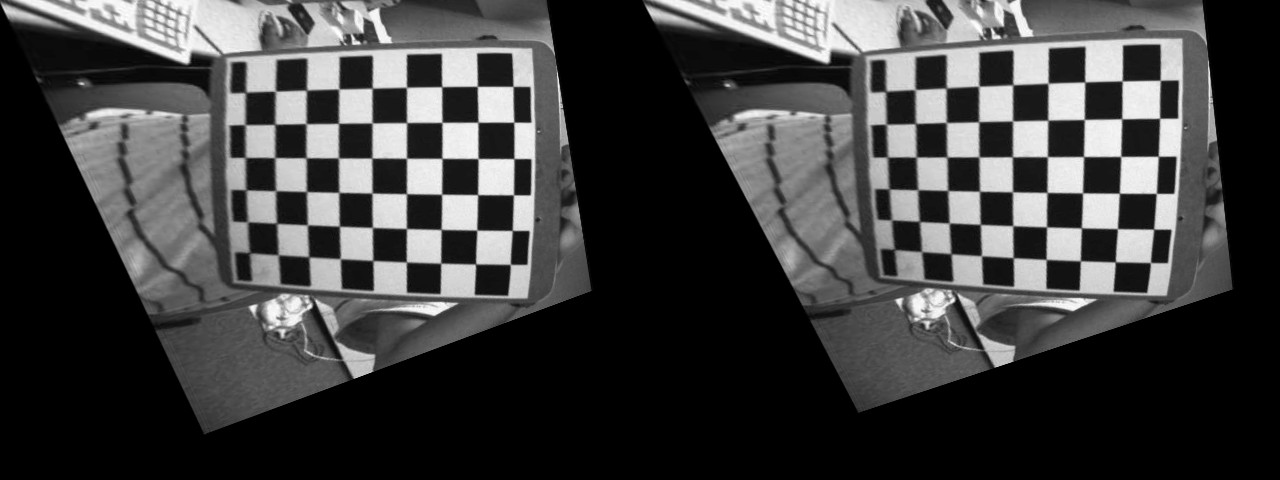
结果图像为：

计算源角点经单应性矩阵变换后的坐标：

为检验计算的正确性，显示了对应的匹配连线：

示例 3：由相机位移求单应性矩阵

单应性矩阵描述了两个平面之间的变换，由此可以恢复出相应的相机位移，使得我们能够从第一个平面视图过渡到第二个平面视图（更多信息见 [Malis2007）。] 在深入介绍如何由相机位移计算单应性矩阵的细节之前，先回顾一下相机位姿与齐次变换。

函数 cv::solvePnP 可以根据 3D 物体点（物体坐标系下的点）与投影的 2D 图像点（在图像中观察到的物体点）之间的对应关系来计算相机位姿。 需要提供内参与畸变系数（参见相机标定过程）。

$$\begin{align*} s \begin{bmatrix} u \\ v \\ 1 \end{bmatrix} &= \begin{bmatrix} f_x & 0 & c_x \\ 0 & f_y & c_y \\ 0 & 0 & 1 \end{bmatrix} \begin{bmatrix} r_{11} & r_{12} & r_{13} & t_x \\ r_{21} & r_{22} & r_{23} & t_y \\ r_{31} & r_{32} & r_{33} & t_z \end{bmatrix} \begin{bmatrix} X_o \\ Y_o \\ Z_o \\ 1 \end{bmatrix} \\ &= \mathbf{K} \hspace{0.2em} ^{c}\mathbf{M}_o \begin{bmatrix} X_o \\ Y_o \\ Z_o \\ 1 \end{bmatrix} \end{align*}$$

$\mathbf{K}$ 是内参矩阵，$^{c}\mathbf{M}_o$ 是相机位姿。cv::solvePnP 的输出正是如此：rvec 是 Rodrigues 旋转向量，tvec 是平移向量。

$^{c}\mathbf{M}_o$ 可以用齐次形式表示，用于将物体坐标系下的点变换到相机坐标系：

$$\begin{align*} \begin{bmatrix} X_c \\ Y_c \\ Z_c \\ 1 \end{bmatrix} &= \hspace{0.2em} ^{c}\mathbf{M}_o \begin{bmatrix} X_o \\ Y_o \\ Z_o \\ 1 \end{bmatrix} \\ &= \begin{bmatrix} ^{c}\mathbf{R}_o & ^{c}\mathbf{t}_o \\ 0_{1\times3} & 1 \end{bmatrix} \begin{bmatrix} X_o \\ Y_o \\ Z_o \\ 1 \end{bmatrix} \\ &= \begin{bmatrix} r_{11} & r_{12} & r_{13} & t_x \\ r_{21} & r_{22} & r_{23} & t_y \\ r_{31} & r_{32} & r_{33} & t_z \\ 0 & 0 & 0 & 1 \end{bmatrix} \begin{bmatrix} X_o \\ Y_o \\ Z_o \\ 1 \end{bmatrix} \end{align*}$$

将一个坐标系下的点变换到另一个坐标系，可以用矩阵乘法轻松完成：

• $^{c_1}\mathbf{M}_o$ 是相机 1 的相机位姿
• $^{c_2}\mathbf{M}_o$ 是相机 2 的相机位姿

将相机 1 坐标系下的 3D 点变换到相机 2 坐标系：

$$^{c_2}\mathbf{M}_{c_1} = \hspace{0.2em} ^{c_2}\mathbf{M}_{o} \cdot \hspace{0.1em} ^{o}\mathbf{M}_{c_1} = \hspace{0.2em} ^{c_2}\mathbf{M}_{o} \cdot \hspace{0.1em} \left( ^{c_1}\mathbf{M}_{o} \right )^{-1} = \begin{bmatrix} ^{c_2}\mathbf{R}_{o} & ^{c_2}\mathbf{t}_{o} \\ 0_{3 \times 1} & 1 \end{bmatrix} \cdot \begin{bmatrix} ^{c_1}\mathbf{R}_{o}^T & - \hspace{0.2em} ^{c_1}\mathbf{R}_{o}^T \cdot \hspace{0.2em} ^{c_1}\mathbf{t}_{o} \\ 0_{1 \times 3} & 1 \end{bmatrix}$$

在本示例中，我们将计算相对于棋盘物体的两个相机位姿之间的相机位移。第一步是计算两幅图像的相机位姿：

相机位移可以由上述公式从相机位姿计算得到：

由相机位移计算得到的、与特定平面相关的单应性矩阵为：

在此图中，n 是平面的法向量，d 是沿平面法线方向相机坐标系与平面之间的距离。 计算由相机位移得到单应性矩阵的方程为：

$$^{2}\mathbf{H}_{1} = \hspace{0.2em} ^{2}\mathbf{R}_{1} - \hspace{0.1em} \frac{^{2}\mathbf{t}_{1} \cdot \hspace{0.1em} ^{1}\mathbf{n}^\top}{^1d}$$

其中 $^{2}\mathbf{H}_{1}$ 是将第一个相机坐标系中的点映射到第二个相机坐标系中对应点的单应性矩阵， $^{2}\mathbf{R}_{1} = \hspace{0.2em} ^{c_2}\mathbf{R}_{o} \cdot \hspace{0.1em} ^{c_1}\mathbf{R}_{o}^{\top}$ 是表示两个相机坐标系之间旋转的旋转矩阵， 而 $^{2}\mathbf{t}_{1} = \hspace{0.2em} ^{c_2}\mathbf{R}_{o} \cdot \left( - \hspace{0.1em} ^{c_1}\mathbf{R}_{o}^{\top} \cdot \hspace{0.1em} ^{c_1}\mathbf{t}_{o} \right ) + \hspace{0.1em} ^{c_2}\mathbf{t}_{o}$ 是两个相机坐标系之间的平移向量。

这里的法向量 n 是在相机坐标系 1 中表示的平面法向量，可以用两个向量的叉积（使用平面上 3 个不共线的点）计算，在本例中则直接用：

距离 d 可以用平面法向量与平面上某一点的点积来计算，也可以通过计算平面方程并使用其中的 D 系数来计算：

投影单应性矩阵 $\textbf{G}$ 可由欧氏单应性矩阵 $\textbf{H}$ 通过内参矩阵 $\textbf{K}$ 计算得到（见 [Malis2007），这里假设两个平面视图之间是同一相机：]

$$\textbf{G} = \gamma \textbf{K} \textbf{H} \textbf{K}^{-1}$$

在我们的情形中，棋盘的 Z 轴指向物体内部，而单应性矩阵示意图中的 Z 轴指向外部。这只是符号的问题：

$$^{2}\mathbf{H}_{1} = \hspace{0.2em} ^{2}\mathbf{R}_{1} + \hspace{0.1em} \frac{^{2}\mathbf{t}_{1} \cdot \hspace{0.1em} ^{1}\mathbf{n}^\top}{^1d}$$

现在，我们将由相机位移计算得到的投影单应性矩阵，与用 cv::findHomography 估计出的单应性矩阵进行比较。

findHomography H:
[0.32903393332201, -1.244138808862929, 536.4769088231476;
 0.6969763913334046, -0.08935909072571542, -80.34068504082403;
 0.00040511729592961, -0.001079740100565013, 0.9999999999999999]

homography from camera displacement:
[0.4160569997384721, -1.306889006892538, 553.7055461075881;
 0.7917584252773352, -0.06341244158456338, -108.2770029401219;
 0.0005926357240956578, -0.001020651672127799, 1]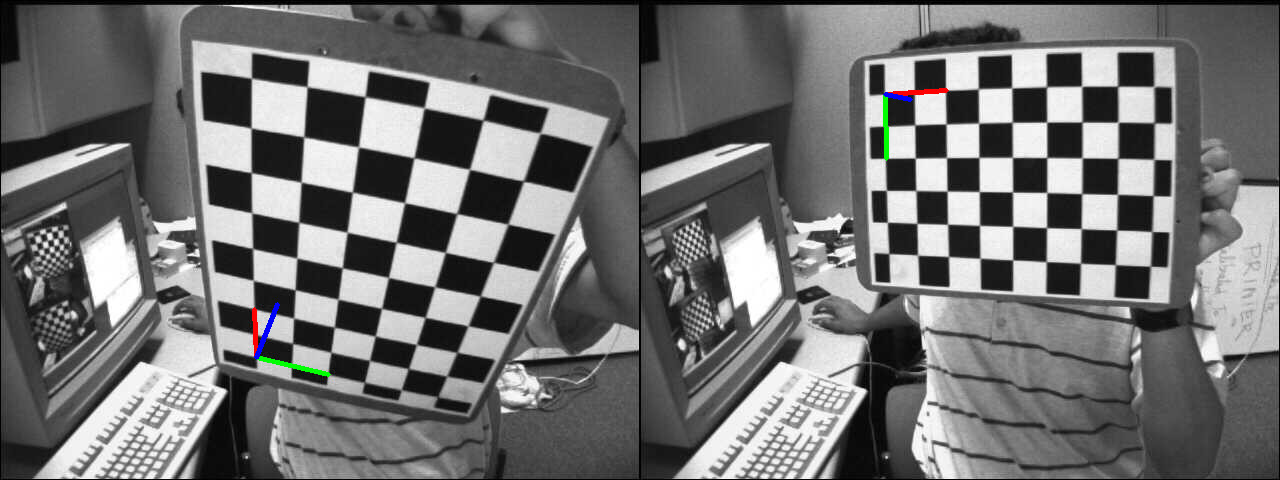

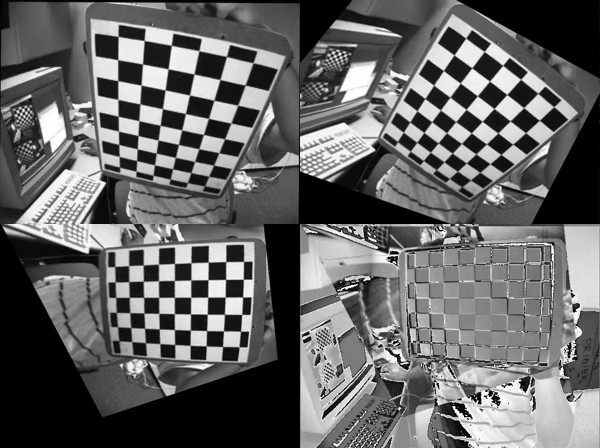
这两个单应性矩阵是相近的。如果我们比较分别用这两个单应性矩阵对图像 1 做变换后的结果：

从视觉上看，很难区分由相机位移计算的单应性矩阵所得结果图像与用 cv::findHomography 函数估计的单应性矩阵所得结果图像之间的差别。

练习

本示例展示了如何从两个相机位姿计算单应性变换。请尝试完成同样的操作，但这次改为计算 N 个中间单应性矩阵。 与其计算一个单应性矩阵直接将源图像变换到目标相机视角，不如执行 N 次变换操作，以观察不同变换的效果。

你应该会得到与下图类似的结果：

示例 4：分解单应性矩阵

OpenCV 3 包含函数 cv::decomposeHomographyMat，它可以将单应性矩阵分解为一组旋转、平移与平面法向量。 首先，我们分解由相机位移计算得到的单应性矩阵：

cv::decomposeHomographyMat 的结果为：

Solution 0:
rvec from homography decomposition: [-0.0919829920641369, -0.5372581036567992, 1.310868863540717]
rvec from camera displacement: [-0.09198299206413783, -0.5372581036567995, 1.310868863540717]
tvec from homography decomposition: [-0.7747961019053186, -0.02751124463434032, -0.6791980037590677] and scaled by d: [-0.1578091561210742, -0.005603443652993778, -0.1383378976078466]
tvec from camera displacement: [0.1578091561210745, 0.005603443652993617, 0.1383378976078466]
plane normal from homography decomposition: [-0.1973513139420648, 0.6283451996579074, -0.7524857267431757]
plane normal at camera 1 pose: [0.1973513139420654, -0.6283451996579068, 0.752485726743176]

Solution 1:
rvec from homography decomposition: [-0.0919829920641369, -0.5372581036567992, 1.310868863540717]
rvec from camera displacement: [-0.09198299206413783, -0.5372581036567995, 1.310868863540717]
tvec from homography decomposition: [0.7747961019053186, 0.02751124463434032, 0.6791980037590677] and scaled by d: [0.1578091561210742, 0.005603443652993778, 0.1383378976078466]
tvec from camera displacement: [0.1578091561210745, 0.005603443652993617, 0.1383378976078466]
plane normal from homography decomposition: [0.1973513139420648, -0.6283451996579074, 0.7524857267431757]
plane normal at camera 1 pose: [0.1973513139420654, -0.6283451996579068, 0.752485726743176]

Solution 2:
rvec from homography decomposition: [0.1053487907109967, -0.1561929144786397, 1.401356552358475]
rvec from camera displacement: [-0.09198299206413783, -0.5372581036567995, 1.310868863540717]
tvec from homography decomposition: [-0.4666552552894618, 0.1050032934770042, -0.913007654671646] and scaled by d: [-0.0950475510338766, 0.02138689274867372, -0.1859598508065552]
tvec from camera displacement: [0.1578091561210745, 0.005603443652993617, 0.1383378976078466]
plane normal from homography decomposition: [-0.3131715472900788, 0.8421206145721947, -0.4390403768225507]
plane normal at camera 1 pose: [0.1973513139420654, -0.6283451996579068, 0.752485726743176]

Solution 3:
rvec from homography decomposition: [0.1053487907109967, -0.1561929144786397, 1.401356552358475]
rvec from camera displacement: [-0.09198299206413783, -0.5372581036567995, 1.310868863540717]
tvec from homography decomposition: [0.4666552552894618, -0.1050032934770042, 0.913007654671646] and scaled by d: [0.0950475510338766, -0.02138689274867372, 0.1859598508065552]
tvec from camera displacement: [0.1578091561210745, 0.005603443652993617, 0.1383378976078466]
plane normal from homography decomposition: [0.3131715472900788, -0.8421206145721947, 0.4390403768225507]
plane normal at camera 1 pose: [0.1973513139420654, -0.6283451996579068, 0.752485726743176]

单应性矩阵分解的结果只能相差一个尺度因子恢复出来，该尺度因子实际上就对应于距离 d，因为法向量是单位长度的。 如你所见，有一个解与计算出的相机位移几乎完全吻合。正如文档中所述：

At least two of the solutions may further be invalidated if point correspondences are available by applying positive depth constraint (all points must be in front of the camera).

由于分解的结果是一个相机位移，如果我们有初始相机位姿 $^{c_1}\mathbf{M}_{o}$，就可以计算当前相机位姿 $^{c_2}\mathbf{M}_{o} = \hspace{0.2em} ^{c_2}\mathbf{M}_{c_1} \cdot \hspace{0.1em} ^{c_1}\mathbf{M}_{o}$， 并测试属于该平面的 3D 物体点是否投影在相机前方。 另一种方案是，如果我们已知相机位姿 1 处的平面法向量，可以保留法向量最接近的那个解。

下面是用 cv::findHomography 估计出的单应性矩阵做同样处理：

Solution 0:
rvec from homography decomposition: [0.1552207729599141, -0.152132696119647, 1.323678695078694]
rvec from camera displacement: [-0.09198299206413783, -0.5372581036567995, 1.310868863540717]
tvec from homography decomposition: [-0.4482361704818117, 0.02485247635491922, -1.034409687207331] and scaled by d: [-0.09129598307571339, 0.005061910238634657, -0.2106868109173855]
tvec from camera displacement: [0.1578091561210745, 0.005603443652993617, 0.1383378976078466]
plane normal from homography decomposition: [-0.1384902722707529, 0.9063331452766947, -0.3992250922214516]
plane normal at camera 1 pose: [0.1973513139420654, -0.6283451996579068, 0.752485726743176]

Solution 1:
rvec from homography decomposition: [0.1552207729599141, -0.152132696119647, 1.323678695078694]

rvec from camera displacement: [-0.09198299206413783, -0.5372581036567995, 1.310868863540717]
tvec from homography decomposition: [0.4482361704818117, -0.02485247635491922, 1.034409687207331] and scaled by d: [0.09129598307571339, -0.005061910238634657, 0.2106868109173855]
tvec from camera displacement: [0.1578091561210745, 0.005603443652993617, 0.1383378976078466]
plane normal from homography decomposition: [0.1384902722707529, -0.9063331452766947, 0.3992250922214516]
plane normal at camera 1 pose: [0.1973513139420654, -0.6283451996579068, 0.752485726743176]

Solution 2:
rvec from homography decomposition: [-0.2886605671759886, -0.521049903923871, 1.381242030882511]
rvec from camera displacement: [-0.09198299206413783, -0.5372581036567995, 1.310868863540717]
tvec from homography decomposition: [-0.8705961357284295, 0.1353018038908477, -0.7037702049789747] and scaled by d: [-0.177321544550518, 0.02755804196893467, -0.1433427218822783]
tvec from camera displacement: [0.1578091561210745, 0.005603443652993617, 0.1383378976078466]
plane normal from homography decomposition: [-0.2284582117722427, 0.6009247303964522, -0.7659610393954643]
plane normal at camera 1 pose: [0.1973513139420654, -0.6283451996579068, 0.752485726743176]

Solution 3:
rvec from homography decomposition: [-0.2886605671759886, -0.521049903923871, 1.381242030882511]
rvec from camera displacement: [-0.09198299206413783, -0.5372581036567995, 1.310868863540717]
tvec from homography decomposition: [0.8705961357284295, -0.1353018038908477, 0.7037702049789747] and scaled by d: [0.177321544550518, -0.02755804196893467, 0.1433427218822783]
tvec from camera displacement: [0.1578091561210745, 0.005603443652993617, 0.1383378976078466]
plane normal from homography decomposition: [0.2284582117722427, -0.6009247303964522, 0.7659610393954643]
plane normal at camera 1 pose: [0.1973513139420654, -0.6283451996579068, 0.752485726743176]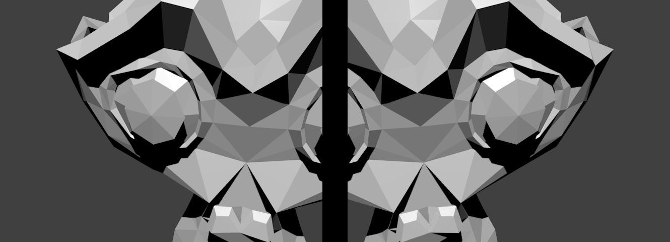

同样，这里也有一个解与计算出的相机位移相吻合。

示例 5：旋转相机的基础全景拼接

\note 本示例旨在说明基于相机纯旋转运动的图像拼接概念，不应用于拼接全景图像。 stitching 模块 提供了完整的图像拼接流水线。

单应性变换仅适用于平面结构。但在相机旋转的情况下（绕相机投影轴的纯旋转，无平移），可以将任意场景视为平面 （见前文）。

此时单应性矩阵可以用旋转变换与相机内参计算得到（例如见 \ref homography_course “10”）：

$$s \begin{bmatrix} x^{'} \\ y^{'} \\ 1 \end{bmatrix} = \bf{K} \hspace{0.1em} \bf{R} \hspace{0.1em} \bf{K}^{-1} \begin{bmatrix} x \\ y \\ 1 \end{bmatrix}$$

为了说明这一点，我们使用 Blender（一款自由开源的 3D 计算机图形软件）生成了两个仅有旋转变换的相机视图。 关于如何用 Blender 获取相机内参与相对于世界坐标系的 3x4 外参矩阵的更多信息，可参见 \ref answer_blender “11”（需要额外一次变换才能得到相机坐标系与物体坐标系之间的变换）。

下图展示了 Suzanne 模型的两个视图，二者之间仅有旋转变换：

已知对应的相机位姿与内参，就可以计算出两个视图之间的相对旋转：

这里，第二幅图像将相对于第一幅图像进行拼接。单应性矩阵可以用上述公式计算：

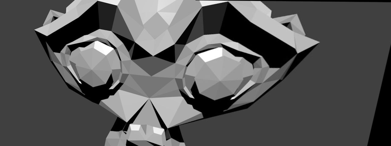
拼接简单地用以下方式完成：

结果图像为：

补充参考文献

• \anchor lecture_16 1. Lecture 16: Planar Homographies，Robert Collins
• \anchor projective_transformations 2. 2D projective transformations (homographies)，Christiano Gava、Gabriele Bleser
• \anchor szeliski 3. Computer Vision: Algorithms and Applications，Richard Szeliski
• \anchor answer_dsp 4. Step by Step Camera Pose Estimation for Visual Tracking and Planar Markers
• \anchor pose_ar 5. Pose from homography estimation
• \anchor polar_decomposition 6. Polar Decomposition (in Continuum Mechanics)
• \anchor polar_decomposition_svd 7. Chapter 3 - 3.1.2 From matrices to rotations - Theorem 3.1 (Least-squares estimation of a rotation from a matrix K)
• \anchor polar_decomposition_svd_2 8. A Personal Interview with the Singular Value Decomposition，Matan Gavish
• \anchor Kabsch_algorithm 9. Kabsch algorithm, Computation of the optimal rotation matrix
• \anchor homography_course 10. Homography，Dr. Gerhard Roth
• \anchor answer_blender 11. 3x4 camera matrix from blender camera