基于梯度结构张量的各向异性图像分割

本教程中你将学到：

什么是梯度结构张量（gradient structure tensor）
如何用梯度结构张量估计各向异性图像的取向（orientation）与相干性（coherency）
如何用梯度结构张量对具有单一局部取向的各向异性图像进行分割

理论

注意： 本说明基于书籍 Computer Vision and Applications（Jähne, 2000）、Vision Foundations（Bigun, 2006）与 Van Vliet and Verbeek (1995) 的相关章节。Yang（1996）对梯度结构张量给出了很好的物理解释。此外，你也可以参考维基百科页面 Structure tensor。

注意： 本页所讨论的各向异性图像均为真实世界图像。

什么是梯度结构张量？

在数学中，梯度结构张量（也称为二阶矩矩阵、二阶矩张量、惯性张量等）是由函数梯度导出的一个矩阵。它概括了在某点指定邻域内梯度占主导的方向，以及这些方向相干的程度（coherency，相干性）。梯度结构张量广泛应用于图像处理与计算机视觉中的二维/三维图像分割、运动检测、自适应滤波、局部图像特征检测等领域。

各向异性图像的重要特征包括局部各向异性的取向与相干性。本文将说明如何估计取向与相干性，以及如何用梯度结构张量分割具有单一局部取向的各向异性图像。

图像的梯度结构张量是一个 2×2 对称矩阵。梯度结构张量的特征向量指示局部取向，而特征值给出相干性（各向异性程度的度量）。

图像 $Z$ 的梯度结构张量 $J$ 可写为：

$J = \begin{bmatrix} J_{11} & J_{12} \\ J_{12} & J_{22} \end{bmatrix}$

其中 $J_{11} = M[Z_{x}^{2}]$ 、 $J_{22} = M[Z_{y}^{2}]$ 、 $J_{12} = M[Z_{x}Z_{y}]$ 为张量的分量， $M[]$ 表示数学期望（我们可以把这一运算视作在窗口 w 内取平均）， $Z_{x}$ 与 $Z_{y}$ 是图像 $Z$ 关于 $x$ 与 $y$ 的偏导数。

该张量的特征值可由下式求得：

$\lambda_{1,2} = \frac{1}{2} \left [ J_{11} + J_{22} \pm \sqrt{(J_{11} - J_{22})^{2} + 4J_{12}^{2}} \right ]$

其中 $\lambda_1$ 为最大特征值， $\lambda_2$ 为最小特征值。

如何用梯度结构张量估计各向异性图像的取向与相干性？

各向异性图像的取向：

$\alpha = 0.5\,\mathrm{arctan}\frac{2J_{12}}{J_{22} - J_{11}}$

相干性：

$C = \frac{\lambda_1 - \lambda_2}{\lambda_1 + \lambda_2}$

相干性取值范围为 0 到 1。对于理想的局部取向（ $\lambda_2 = 0$ ， $\lambda_1 > 0$ ），相干性为 1；对于各向同性的灰度值结构（ $\lambda_1 = \lambda_2 > 0$ ），相干性为 0。

源代码

你可以在 OpenCV 源码库的 samples/cpp/tutorial_code/ImgProc/anisotropic_image_segmentation/anisotropic_image_segmentation.cpp 中找到源代码，也可下载 C++ 版本或 Python 版本。

说明

各向异性图像分割算法由梯度结构张量计算、取向计算、相干性计算以及取向与相干性阈值化处理组成：

函数 calcGST() 利用梯度结构张量计算取向与相干性。输入参数 w 定义了窗口大小：

void calcGST(const Mat& inputImg, Mat& imgCoherencyOut, Mat& imgOrientationOut, int w)
{
    Mat img;
    inputImg.convertTo(img, CV_32F);

    // GST components calculation (start)
    // J =  (J11 J12; J12 J22) - GST
    Mat imgDiffX, imgDiffY, imgDiffXY;
    Sobel(img, imgDiffX, CV_32F, 1, 0, 3);
    Sobel(img, imgDiffY, CV_32F, 0, 1, 3);
    multiply(imgDiffX, imgDiffY, imgDiffXY);

    Mat imgDiffXX, imgDiffYY;
    multiply(imgDiffX, imgDiffX, imgDiffXX);
    multiply(imgDiffY, imgDiffY, imgDiffYY);

    Mat J11, J22, J12;      // J11, J22 and J12 are GST components
    boxFilter(imgDiffXX, J11, CV_32F, Size(w, w));
    boxFilter(imgDiffYY, J22, CV_32F, Size(w, w));
    boxFilter(imgDiffXY, J12, CV_32F, Size(w, w));
    // GST components calculation (stop)

    // eigenvalue calculation (start)
    // lambda1 = 0.5*(J11 + J22 + sqrt((J11-J22)^2 + 4*J12^2))
    // lambda2 = 0.5*(J11 + J22 - sqrt((J11-J22)^2 + 4*J12^2))
    Mat tmp1, tmp2, tmp3, tmp4;
    tmp1 = J11 + J22;
    tmp2 = J11 - J22;
    multiply(tmp2, tmp2, tmp2);
    multiply(J12, J12, tmp3);
    sqrt(tmp2 + 4.0 * tmp3, tmp4);

    Mat lambda1, lambda2;
    lambda1 = tmp1 + tmp4;
    lambda1 = 0.5*lambda1;      // biggest eigenvalue
    lambda2 = tmp1 - tmp4;
    lambda2 = 0.5*lambda2;      // smallest eigenvalue
    // eigenvalue calculation (stop)

    // Coherency calculation (start)
    // Coherency = (lambda1 - lambda2)/(lambda1 + lambda2)) - measure of anisotropism
    // Coherency is anisotropy degree (consistency of local orientation)
    divide(lambda1 - lambda2, lambda1 + lambda2, imgCoherencyOut);
    // Coherency calculation (stop)

    // orientation angle calculation (start)
    // tan(2*alpha) = 2*J12/(J22 - J11)
    // alpha = 0.5*atan2(2*J12, J22 - J11)
    phase(J22 - J11, 2.0*J12, imgOrientationOut, true);
    imgOrientationOut = 0.5*imgOrientationOut;
    // orientation angle calculation (stop)
}

下面的代码对前一函数计算出的图像取向应用阈值 LowThr 与 HighThr，对图像相干性应用阈值 C_Thr。LowThr 与 HighThr 定义了取向范围：

Mat imgCoherencyBin;
imgCoherencyBin = imgCoherency > C_Thr;
Mat imgOrientationBin;
inRange(imgOrientation, Scalar(LowThr), Scalar(HighThr), imgOrientationBin);

最后，我们将阈值化结果合并：

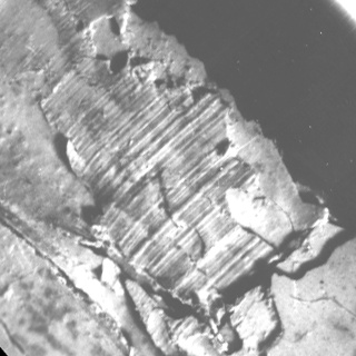
Mat imgBin;
imgBin = imgCoherencyBin & imgOrientationBin;

结果

下图是具有单一方向的真实各向异性图像：

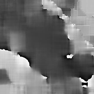
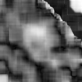
下图是该各向异性图像的取向与相干性：

下图是分割结果：

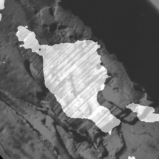
该结果使用 w = 52、C_Thr = 0.43、LowThr = 35、HighThr = 57 计算得到。可以看到，算法只选取了具有单一方向的区域。

参考文献

Jähne, B. Computer Vision and Applications（2000）
Bigun, J. Vision Foundations（2006）
Van Vliet, L. J., & Verbeek, P. W. Estimators for orientation and anisotropy in digitized images（1995）
Yang, Z. Structure tensor analysis（1996）
Structure tensor —— 维基百科上关于结构张量的描述