霍夫线变换

目标

在本教程中，你将学到：

如何使用 OpenCV 函数 HoughLines() 和 HoughLinesP() 来检测图像中的直线。

原理

霍夫线变换（Hough Line Transform）

霍夫线变换是一种用于检测直线的变换。
在应用该变换之前，最好先进行边缘检测预处理。

它是如何工作的？

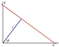
如你所知，图像空间中的一条直线可以用两个变量来表示。例如：
1. 在笛卡尔坐标系中：参数为 $(m,b)$ 。
2. 在极坐标系中：参数为 $(r,\theta)$
对于霍夫变换，我们将在极坐标系中表达直线。因此，直线方程可以写为：

$y = \left ( -\dfrac{\cos \theta}{\sin \theta} \right ) x + \left ( \dfrac{r}{\sin \theta} \right )$

整理各项可得： $r = x \cos \theta + y \sin \theta$
一般来说，对于每个点 $(x_{0}, y_{0})$ ，我们可以把经过该点的一族直线定义为：

$r_{\theta} = x_{0} \cdot \cos \theta + y_{0} \cdot \sin \theta$

也就是说，每一对 $(r_{\theta},\theta)$ 都代表一条经过 $(x_{0}, y_{0})$ 的直线。
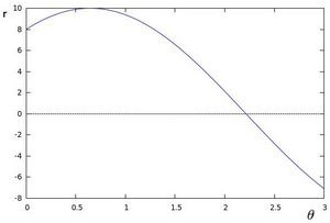
如果对给定的 $(x_{0}, y_{0})$ 画出经过它的那一族直线，我们会得到一条正弦曲线。例如，对于 $x_{0} = 8$ 、 $y_{0} = 6$ ，我们得到如下曲线（在 $\theta$ - $r$ 平面上）：

我们只考虑满足 $r > 0$ 且 $0< \theta < 2 \pi$ 的点。
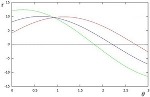
我们可以对图像中的所有点执行同样的操作。如果两个不同点的曲线在 $\theta$ - $r$ 平面中相交，就意味着这两个点属于同一条直线。例如，继续上面的例子，再为两个点 $x_{1} = 4$ 、 $y_{1} = 9$ 和 $x_{2} = 12$ 、 $y_{2} = 3$ 画出曲线，我们得到：

三条曲线相交于同一个点 $(0.925, 9.6)$ ，这些坐标就是 $(x_{0}, y_{0})$ 、 $(x_{1}, y_{1})$ 和 $(x_{2}, y_{2})$ 所在直线的参数（ $\theta, r$ ）。
上面这一切意味着什么？它意味着，一般来说，一条直线可以通过找出曲线之间的交点数量来被检测出来。相交的曲线越多，说明该交点所代表的直线上的点就越多。一般来说，我们可以定义一个阈值，表示检测一条直线所需的最少交点数量。
这正是霍夫线变换所做的事情。它跟踪图像中每个点的曲线之间的交点。如果交点数量超过某个阈值，就把它判定为一条直线，其参数就是交点的 $(\theta, r_{\theta})$ 。

标准霍夫变换与概率霍夫变换

OpenCV 实现了三种霍夫线变换：

a. 标准霍夫变换（Standard Hough Transform）

基本就是我们上一节讲解的内容。它给出的结果是一个由 $(\theta, r_{\theta})$ 对组成的向量。
在 OpenCV 中由函数 HoughLines() 实现。

b. 概率霍夫线变换（Probabilistic Hough Line Transform）

霍夫线变换的一种更高效的实现。它输出检测到的直线的两个端点 $(x_{0}, y_{0}, x_{1}, y_{1})$ 。
在 OpenCV 中由函数 HoughLinesP() 实现。

c. 加权霍夫变换（Weighted Hough Transform）

使用边缘强度值，而不是标准霍夫变换中的二值 0 或 1。
在 OpenCV 中由函数 HoughLines() 配合 use_edgeval=true 实现。
示例见 samples/cpp/tutorial_code/ImgTrans/HoughLines_Demo.cpp。

本程序做什么？

加载一幅图像；
应用一次标准霍夫线变换和一次概率霍夫线变换；
在三个窗口中显示原图和检测到的直线。

代码

C++：

我们将要讲解的示例代码可以从这里下载。一个稍复杂一点的版本（同时展示标准与概率霍夫变换，并带有用于调整阈值的 Trackbar）可以在这里找到。

/**
 * @file houghlines.cpp
 * @brief This program demonstrates line finding with the Hough transform
 */

#include "opencv2/imgcodecs.hpp"
#include "opencv2/highgui.hpp"
#include "opencv2/imgproc.hpp"

using namespace cv;
using namespace std;

int main(int argc, char** argv)
{
    // Declare the output variables
    Mat dst, cdst, cdstP;

    const char* default_file = "sudoku.png";
    const char* filename = argc >=2 ? argv[1] : default_file;

    // Loads an image
    Mat src = imread( samples::findFile( filename ), IMREAD_GRAYSCALE );

    // Check if image is loaded fine
    if(src.empty()){
        printf(" Error opening image\n");
        printf(" Program Arguments: [image_name -- default %s] \n", default_file);
        return -1;
    }

    // Edge detection
    Canny(src, dst, 50, 200, 3);

    // Copy edges to the images that will display the results in BGR
    cvtColor(dst, cdst, COLOR_GRAY2BGR);
    cdstP = cdst.clone();

    // Standard Hough Line Transform
    vector<Vec2f> lines; // will hold the results of the detection
    HoughLines(dst, lines, 1, CV_PI/180, 150, 0, 0 ); // runs the actual detection
    // Draw the lines
    for( size_t i = 0; i < lines.size(); i++ )
    {
        float rho = lines[i][0], theta = lines[i][1];
        Point pt1, pt2;
        double a = cos(theta), b = sin(theta);
        double x0 = a*rho, y0 = b*rho;
        pt1.x = cvRound(x0 + 1000*(-b));
        pt1.y = cvRound(y0 + 1000*(a));
        pt2.x = cvRound(x0 - 1000*(-b));
        pt2.y = cvRound(y0 - 1000*(a));
        line( cdst, pt1, pt2, Scalar(0,0,255), 3, LINE_AA);
    }

    // Probabilistic Line Transform
    vector<Vec4i> linesP; // will hold the results of the detection
    HoughLinesP(dst, linesP, 1, CV_PI/180, 50, 50, 10 ); // runs the actual detection
    // Draw the lines
    for( size_t i = 0; i < linesP.size(); i++ )
    {
        Vec4i l = linesP[i];
        line( cdstP, Point(l[0], l[1]), Point(l[2], l[3]), Scalar(0,0,255), 3, LINE_AA);
    }

    // Show results
    imshow("Source", src);
    imshow("Detected Lines (in red) - Standard Hough Line Transform", cdst);
    imshow("Detected Lines (in red) - Probabilistic Line Transform", cdstP);

    // Wait and Exit
    waitKey();
    return 0;
}

Java：

我们将要讲解的示例代码可以从这里下载。

/**
 * @file HoughLines.java
 * @brief This program demonstrates line finding with the Hough transform
 */

import org.opencv.core.*;
import org.opencv.core.Point;
import org.opencv.highgui.HighGui;
import org.opencv.imgcodecs.Imgcodecs;
import org.opencv.imgproc.Imgproc;

class HoughLinesRun {

    public void run(String[] args) {
        // Declare the output variables
        Mat dst = new Mat(), cdst = new Mat(), cdstP;

        String default_file = "../../../../data/sudoku.png";
        String filename = ((args.length > 0) ? args[0] : default_file);

        // Load an image
        Mat src = Imgcodecs.imread(filename, Imgcodecs.IMREAD_GRAYSCALE);

        // Check if image is loaded fine
        if( src.empty() ) {
            System.out.println("Error opening image!");
            System.out.println("Program Arguments: [image_name -- default "
                    + default_file +"] \n");
            System.exit(-1);
        }

        // Edge detection
        Imgproc.Canny(src, dst, 50, 200, 3, false);

        // Copy edges to the images that will display the results in BGR
        Imgproc.cvtColor(dst, cdst, Imgproc.COLOR_GRAY2BGR);
        cdstP = cdst.clone();

        // Standard Hough Line Transform
        Mat lines = new Mat(); // will hold the results of the detection
        Imgproc.HoughLines(dst, lines, 1, Math.PI/180, 150); // runs the actual detection
        // Draw the lines
        for (int x = 0; x < lines.rows(); x++) {
            double rho = lines.get(x, 0)[0],
                    theta = lines.get(x, 0)[1];

            double a = Math.cos(theta), b = Math.sin(theta);
            double x0 = a*rho, y0 = b*rho;
            Point pt1 = new Point(Math.round(x0 + 1000*(-b)), Math.round(y0 + 1000*(a)));
            Point pt2 = new Point(Math.round(x0 - 1000*(-b)), Math.round(y0 - 1000*(a)));
            Imgproc.line(cdst, pt1, pt2, new Scalar(0, 0, 255), 3, Imgproc.LINE_AA, 0);
        }

        // Probabilistic Line Transform
        Mat linesP = new Mat(); // will hold the results of the detection
        Imgproc.HoughLinesP(dst, linesP, 1, Math.PI/180, 50, 50, 10); // runs the actual detection
        // Draw the lines
        for (int x = 0; x < linesP.rows(); x++) {
            double[] l = linesP.get(x, 0);
            Imgproc.line(cdstP, new Point(l[0], l[1]), new Point(l[2], l[3]), new Scalar(0, 0, 255), 3, Imgproc.LINE_AA, 0);
        }

        // Show results
        HighGui.imshow("Source", src);
        HighGui.imshow("Detected Lines (in red) - Standard Hough Line Transform", cdst);
        HighGui.imshow("Detected Lines (in red) - Probabilistic Line Transform", cdstP);

        // Wait and Exit
        HighGui.waitKey();
        System.exit(0);
    }
}

public class HoughLines {
    public static void main(String[] args) {
        // Load the native library.
        System.loadLibrary(Core.NATIVE_LIBRARY_NAME);
        new HoughLinesRun().run(args);
    }
}

Python：

我们将要讲解的示例代码可以从这里下载。

"""
@file hough_lines.py
@brief This program demonstrates line finding with the Hough transform
"""
import sys
import math
import cv2 as cv
import numpy as np


def main(argv):
    default_file = 'sudoku.png'
    filename = argv[0] if len(argv) > 0 else default_file

    # Loads an image
    src = cv.imread(cv.samples.findFile(filename), cv.IMREAD_GRAYSCALE)

    # Check if image is loaded fine
    if src is None:
        print ('Error opening image!')
        print ('Usage: hough_lines.py [image_name -- default ' + default_file + '] \n')
        return -1

    # Edge detection
    dst = cv.Canny(src, 50, 200, None, 3)

    # Copy edges to the images that will display the results in BGR
    cdst = cv.cvtColor(dst, cv.COLOR_GRAY2BGR)
    cdstP = np.copy(cdst)

    #  Standard Hough Line Transform
    lines = cv.HoughLines(dst, 1, np.pi / 180, 150, None, 0, 0)
    # Draw the lines
    if lines is not None:
        for i in range(0, len(lines)):
            rho = lines[i][0][0]
            theta = lines[i][0][1]
            a = math.cos(theta)
            b = math.sin(theta)
            x0 = a * rho
            y0 = b * rho
            pt1 = (int(x0 + 1000*(-b)), int(y0 + 1000*(a)))
            pt2 = (int(x0 - 1000*(-b)), int(y0 - 1000*(a)))

            cv.line(cdst, pt1, pt2, (0,0,255), 3, cv.LINE_AA)

    # Probabilistic Line Transform
    linesP = cv.HoughLinesP(dst, 1, np.pi / 180, 50, None, 50, 10)
    # Draw the lines
    if linesP is not None:
        for i in range(0, len(linesP)):
            l = linesP[i][0]
            cv.line(cdstP, (l[0], l[1]), (l[2], l[3]), (0,0,255), 3, cv.LINE_AA)
    # Show results
    cv.imshow("Source", src)
    cv.imshow("Detected Lines (in red) - Standard Hough Line Transform", cdst)
    cv.imshow("Detected Lines (in red) - Probabilistic Line Transform", cdstP)
    # Wait and Exit
    cv.waitKey()
    return 0

if __name__ == "__main__":
    main(sys.argv[1:])

说明

加载图像

C++：

const char* default_file = "sudoku.png";
const char* filename = argc >=2 ? argv[1] : default_file;

// Loads an image
Mat src = imread( samples::findFile( filename ), IMREAD_GRAYSCALE );

// Check if image is loaded fine
if(src.empty()){
    printf(" Error opening image\n");
    printf(" Program Arguments: [image_name -- default %s] \n", default_file);
    return -1;
}

Java：

String default_file = "../../../../data/sudoku.png";
String filename = ((args.length > 0) ? args[0] : default_file);

// Load an image
Mat src = Imgcodecs.imread(filename, Imgcodecs.IMREAD_GRAYSCALE);

// Check if image is loaded fine
if( src.empty() ) {
    System.out.println("Error opening image!");
    System.out.println("Program Arguments: [image_name -- default "
            + default_file +"] \n");
    System.exit(-1);
}

Python：

default_file = 'sudoku.png'
filename = argv[0] if len(argv) > 0 else default_file

# Loads an image
src = cv.imread(cv.samples.findFile(filename), cv.IMREAD_GRAYSCALE)

# Check if image is loaded fine
if src is None:
    print ('Error opening image!')
    print ('Usage: hough_lines.py [image_name -- default ' + default_file + '] \n')
    return -1

使用 Canny 检测器检测图像的边缘

C++：

// Edge detection
Canny(src, dst, 50, 200, 3);

Java：

// Edge detection
Imgproc.Canny(src, dst, 50, 200, 3, false);

Python：

# Edge detection
dst = cv.Canny(src, 50, 200, None, 3)

现在我们将应用霍夫线变换。我们会讲解如何使用 OpenCV 为此提供的两个函数。

标准霍夫线变换

首先，应用变换：

C++：

// Standard Hough Line Transform
vector<Vec2f> lines; // will hold the results of the detection
HoughLines(dst, lines, 1, CV_PI/180, 150, 0, 0 ); // runs the actual detection

Java：

// Standard Hough Line Transform
Mat lines = new Mat(); // will hold the results of the detection
Imgproc.HoughLines(dst, lines, 1, Math.PI/180, 150); // runs the actual detection

Python：

#  Standard Hough Line Transform
lines = cv.HoughLines(dst, 1, np.pi / 180, 150, None, 0, 0)

其参数含义如下：

dst：边缘检测器的输出。它应该是一幅灰度图（尽管实际上是一幅二值图）。
lines：一个向量，用来存储检测到的直线的参数 $(r,\theta)$ 。
rho：参数 $r$ 的分辨率，以像素为单位。我们使用 1 像素。
theta：参数 $\theta$ 的分辨率，以弧度为单位。我们使用 1 度（即 CV_PI/180）。
threshold：检测一条直线所需的最少交点数量。
srn 和 stn：默认为 0 的参数。更多信息请查阅 OpenCV 参考文档。

然后通过绘制直线来显示结果。

C++：

// Draw the lines
for( size_t i = 0; i < lines.size(); i++ )
{
    float rho = lines[i][0], theta = lines[i][1];
    Point pt1, pt2;
    double a = cos(theta), b = sin(theta);
    double x0 = a*rho, y0 = b*rho;
    pt1.x = cvRound(x0 + 1000*(-b));
    pt1.y = cvRound(y0 + 1000*(a));
    pt2.x = cvRound(x0 - 1000*(-b));
    pt2.y = cvRound(y0 - 1000*(a));
    line( cdst, pt1, pt2, Scalar(0,0,255), 3, LINE_AA);
}

Java：

// Draw the lines
for (int x = 0; x < lines.rows(); x++) {
    double rho = lines.get(x, 0)[0],
            theta = lines.get(x, 0)[1];

    double a = Math.cos(theta), b = Math.sin(theta);
    double x0 = a*rho, y0 = b*rho;
    Point pt1 = new Point(Math.round(x0 + 1000*(-b)), Math.round(y0 + 1000*(a)));
    Point pt2 = new Point(Math.round(x0 - 1000*(-b)), Math.round(y0 - 1000*(a)));
    Imgproc.line(cdst, pt1, pt2, new Scalar(0, 0, 255), 3, Imgproc.LINE_AA, 0);
}

Python：

# Draw the lines
if lines is not None:
    for i in range(0, len(lines)):
        rho = lines[i][0][0]
        theta = lines[i][0][1]
        a = math.cos(theta)
        b = math.sin(theta)
        x0 = a * rho
        y0 = b * rho
        pt1 = (int(x0 + 1000*(-b)), int(y0 + 1000*(a)))
        pt2 = (int(x0 - 1000*(-b)), int(y0 - 1000*(a)))

        cv.line(cdst, pt1, pt2, (0,0,255), 3, cv.LINE_AA)

概率霍夫线变换

首先，应用变换：

C++：

// Probabilistic Line Transform
vector<Vec4i> linesP; // will hold the results of the detection
HoughLinesP(dst, linesP, 1, CV_PI/180, 50, 50, 10 ); // runs the actual detection

Java：

// Probabilistic Line Transform
Mat linesP = new Mat(); // will hold the results of the detection
Imgproc.HoughLinesP(dst, linesP, 1, Math.PI/180, 50, 50, 10); // runs the actual detection

Python：

# Probabilistic Line Transform
linesP = cv.HoughLinesP(dst, 1, np.pi / 180, 50, None, 50, 10)

其参数含义如下：

dst：边缘检测器的输出。它应该是一幅灰度图（尽管实际上是一幅二值图）。
lines：一个向量，用来存储检测到的直线的参数 $(x_{start}, y_{start}, x_{end}, y_{end})$ 。
rho：参数 $r$ 的分辨率，以像素为单位。我们使用 1 像素。
theta：参数 $\theta$ 的分辨率，以弧度为单位。我们使用 1 度（即 CV_PI/180）。
threshold：检测一条直线所需的最少交点数量。
minLineLength：构成一条直线所需的最少点数。点数少于此值的直线会被忽略。
maxLineGap：两个点之间被视为同一条直线的最大间隔。

然后通过绘制直线来显示结果。

C++：

// Draw the lines
for( size_t i = 0; i < linesP.size(); i++ )
{
    Vec4i l = linesP[i];
    line( cdstP, Point(l[0], l[1]), Point(l[2], l[3]), Scalar(0,0,255), 3, LINE_AA);
}

Java：

// Draw the lines
for (int x = 0; x < linesP.rows(); x++) {
    double[] l = linesP.get(x, 0);
    Imgproc.line(cdstP, new Point(l[0], l[1]), new Point(l[2], l[3]), new Scalar(0, 0, 255), 3, Imgproc.LINE_AA, 0);
}

Python：

# Draw the lines
if linesP is not None:
    for i in range(0, len(linesP)):
        l = linesP[i][0]
        cv.line(cdstP, (l[0], l[1]), (l[2], l[3]), (0,0,255), 3, cv.LINE_AA)

显示原图和检测到的直线

C++：

// Show results
imshow("Source", src);
imshow("Detected Lines (in red) - Standard Hough Line Transform", cdst);
imshow("Detected Lines (in red) - Probabilistic Line Transform", cdstP);

Java：

// Show results
HighGui.imshow("Source", src);
HighGui.imshow("Detected Lines (in red) - Standard Hough Line Transform", cdst);
HighGui.imshow("Detected Lines (in red) - Probabilistic Line Transform", cdstP);

Python：

# Show results
cv.imshow("Source", src)
cv.imshow("Detected Lines (in red) - Standard Hough Line Transform", cdst)
cv.imshow("Detected Lines (in red) - Probabilistic Line Transform", cdstP)

等待用户退出程序

C++：

// Wait and Exit
waitKey();
return 0;

Java：

// Wait and Exit
HighGui.waitKey();
System.exit(0);

Python：

# Wait and Exit
cv.waitKey()
return 0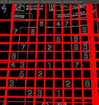

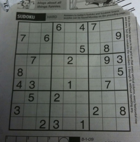
结果

使用一幅输入图像，例如这幅数独图像。使用标准霍夫线变换，我们得到如下结果：

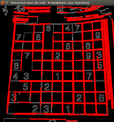
使用概率霍夫线变换，我们得到如下结果：

你可能会观察到，当改变阈值时，检测到的直线数量会发生变化。原因显而易见：阈值设得越高，检测到的直线就越少（因为需要更多的点才能判定一条直线）。